Some common errors when using MPI and OpenMP with FORTRAN

June 5, 2018April 25, 2019 / speedshi / Leave a comment

Error information: Segmentation fault.
Error reason: Stacksize is not enough.
Details: If you declare an array while specifying its dimension at the same time (such as “real :: array(100,100)”), the array will be allocated on the stack. For large arrays, it is recommended to allocate them on the heap rather than on the stack, because the stack size is normally very limited and not very large. Most Fortran compilers implement automatic heap allocation for large arrays. However, when OpenMP is enabled, this auto-allocation feature will be turned off. And for a subroutine, the stacksize has a limited, which does not like the main program that seems do not have a stacksize limitation. So if you are allocating a large array on the stack in a subroutine, this error often happens.
Error solutions: Two ways: 1. Increase the stacksize using: SET OMP_STACKSIZE=xxx M, when running the program. 2. Allocate the array on the heap by first declare and set the array allocatable, then allocate the size of the array.
References: [1] Why Segmentation fault is happening in this openmp code?
[2] Fortran Openmp large array
Error information: Memcpy argument memory ranges overlap. Assertion failed in file helper_fns.c.
Error reason: send buffer and the receive buffer alias in MPI.
Details: When performing communication between different processors, some group communication functions are often used, such as MPI_GATHER, MPI_GATHERV or MPI_SCATTER. When using these functions, if you specify the same address for the send buffer and receiver buffer, then at the root process, the send buffer and the receive buffer alias each other.
Error solutions: Two ways: 1. use different address for the send and receiver buffers. 2. use MPI_IN_PLACE as the send buffer at the root processor.
References: [1] Got error when running MPICH2-1.2.1
[2] MPI_IN_PLACE
Error information: Segmentation fault.
Error reason: forget specify the “ierror” parameter when calling a MPI subroutine in FORTRAN
Details: the calling of MPI subroutines/functions in C and FORTRAN is different. In fortran, the last parameter of a MPI subroutine is normally “ierror”, such as call MPI_Send(buff,n,MPI_REAL,dest,tag,MPI_COMM_WORLD,ierror)
Error solutions: do not forget the “ierror” parameter!
Normally no error information, but you will get horrible results.
Error reason: MPI_Finalize do not work as what you thought.
Error details: the standard MPI instruction only says: MPI_Finalize is used to terminate MPI execution environment. All processes must call this routine before exiting. The number of processes running after this routine is called is undefined; it is best not to perform much more than a return rc after calling MPI_Finalize. But this does not mean all other processors except the root processor 0 terminate. The MPI standard only ask the processor 0 continue to execute after calling MPI_Finalize. The other processors are not explicitly defined. Normally, the compilers will let the other processor still keep executing after they calling MPI_Finalize.
Error solutions: only let the root processor run if you indent to do that after calling MPI_Finalize, such as if (rank==0) then “serial code” end if.
References: [1] MPI_Finalize
[2] MPI_Finalize does not end any processes
Error information: severe (71): integer divide by zero
Possible reason: the data type between MPI and FORTRAN is not consistent
Details: For reasons of portability, MPI predefines its elementary data types. However, for integer parameters, the MPI data type only supports integer(1), integer(2) and integer(4). If you define an integer parameter as the type integer(8) and use this parameter when calling MPI subroutines, you may get this error.
Error solutions: do not using integer(8) to define a MPI integer parameter, such as ‘ierror’, ‘npsize’ and ‘ipsize’.
References: Message Passing Interface (MPI)
Note for using MPI in FORTRAN, please keep the data precision consistent between the FORTRAN data types and MPI data types, such as: MPI_INTEGER4 <-> integer(4) and MPI_REAL8 <-> real(8). If the data types are not match, you may got very wrong results or the program keep run and never ends. One important thing which need specific notice is, for MPI data types in FORTRAN programs, there is NO type to correspond integer(8). So you must avoid passing double precision integer numbers using MPI.
Unformatted stream file is very flexible and powerful. It has good compatibility with other languages such as C. When using Fortran to read and write stream file, we can directly set where to read and write. For example:
——————————————————————————————————
open(unit=10,’filename’,form=’unformatted’,access=’stream’)
write(10,POS=pos_in_bytes) array_write
read(10,POS=pos_in_bytes) array_readin
close(10)
——————————————————————————————————-
We can use POS to specify at which place we want to read or write the data. Note the POS is expressed in Bytes. In Fortran, the file starts from POS=1.
Although in the online tutorials and examples, we can set the POS directly and read the data at any places. But in my cases, when I want to read data segments from a big data file several times using an iteratively way, I can read the first segment correctly, can not read the second segment correctly, and the third segment can be read correctly, but the fourth segment is not OK. Code example:
———————————————————————————————————————
open(unit=10,’filename’,form=’unformatted’,access=’stream’)
do ii=1, n
read(10,POS=8*(ii-1)*offsets+1) array # data is in float, double precision
… …
enddo
close(10)
———————————————————————————————————————–
In the first iteration, the first data segment has been successfully read. But in the second iteration, the second data segment has not been read. It seem that the read commode has not been executed. And the third is OK, the fourth one is not, and so on. I am using MPI in the code as well. But I don’t think this is caused by MPI. But I found solution to this problem. I need to expressively rewind the file after I read it. This problem is still very wired through. Code example:
———————————————————————————————————————
open(unit=10,’filename’,form=’unformatted’,access=’stream’)
do ii=1, n
read(10,POS=8*(ii-1)*offsets+1) array # data is in float, double precision
rewind(10)
… …
enddo
close(10)
———————————————————————————————————————–

Calculating seismic moment

February 20, 2017February 20, 2017 / speedshi / Leave a comment

Seismic moment (M₀) is a quantity used by earthquake seismologists to measure the size of an earthquake. The seismic moment is a measure of the size of an earthquake based on the area of fault rupture, the average amount of slip, and the force that was required to overcome the friction sticking the rocks together that were offset by faulting as shown in figure 1. Seismic moment can also be calculated from the amplitude spectra of seismic waves. The scalar seismic moment M₀ is defined by the equation

$M_{0}=\mu AD$ where μ is the shear modulus of the rocks involved in the earthquake (in Pa, or N/m²), 32 GPa in crust, 75 GPa in mantle; A is the area of the rupture along the geologic fault where the earthquake occurred (in m²); D is the average displacement on A during the rapture (in m) as shown in figure 2.

Figure 1

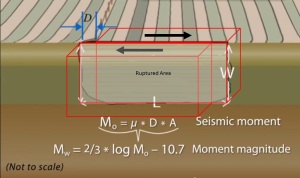
Figure 2

However these information of a rapture are not easy to obtain or estimate in reality. The seismic moment of an earthquake is typically estimated using whatever information is available to constrain its factors. For modern earthquakes, moment is usually estimated from ground motion recordings of earthquakes known as seismograms. For earthquakes that occurred in times before modern instruments were available, moment may be estimated from geologic estimates of the size of the fault rupture and the displacement.

Nowadays seismic moment tensor (M) can be obtained form moment tensor inversion of the recorded seismogram. And the seismic moment (M₀) are defined as the largest absolute eigenvalue of the seismic moment tensor (M)

M₀=max_i(|λ_i|), where λ_i is the eigenvalues of the seismic moment tensor.

Reference:

Earthquake magnitude

February 19, 2017February 19, 2017 / speedshi / Leave a comment

There are different ways to measure an earthquake magnitude.

(1) Richer Magnitude Scale or Local Magnitude Scale (M_L). Richer Magnitude Scale is a base-10 logarithmic scale, which defines magnitude as the logarithm of the ratio of the amplitude of the seismic waves to an arbitrary, minor amplitude, as recorded on a standardized seismograph at a standard distance. It does not apply for earthquakes which have epicentral distance greater than 600 km or magnitude larger than 6.8. Thus it is a local earthquake measurement.

M_L=logA+2.76*logD-2.48, where A is the maximum amplitude recorded on the seismometer in Micrometre, D is the epicentral distance of this seismometer in degree.

(2) Body Wave Magnitude (M_b). Body Wave Magnitude (M_b) is a way of determining the size of an earthquake, using the amplitude of the initial P-wave to calculate the magnitude. Body Wave Magnitude (M_b) does not apply for earthquakes which have an magnitude larger than M_b 6.2.

M_b=log(A/T)+Q(H,D), where A is the maximum amplitude of the first 5s in Micrometre, T is the period of the body wave in second, Q is an empirical term depending on focal depth H and epicentral distance D.

(3) Surface Wave Magnitude (M_s). Surface Wave Magnitude (M_s) is based on measurements in Rayleigh surface waves that travel primarily along the uppermost layers of the Earth. Surface Wave Magnitude (M_s) does not apply for earthquakes which have an magnitude larger than M_s 8.

M_s=log(A/T)+1.66log(D)+3.5, where A is is the maximum particle displacement in surface waves (vector sum of the two horizontal displacements) in Micrometre, T is the corresponding period in second, D is the epicentral distance in degree. There are also some other revised calculation formulas put forward by some other researchers.

(4) Moment Magnitude Scale (M_w). Moment Magnitude Scale (M_w) is used by seismologists to measure the size of earthquakes in terms of the energy released. The magnitude is based on the seismic moment of the earthquake, which is equal to the rigidity of the Earth multiplied by the average amount of slip on the fault and the size of the area that slipped. It can be used to measure big earthquakes.

M_w=2/3log(M0)-10.73, where the M0 is seismic moment in dyne⋅cm (10⁻⁷ N⋅m). The constant values in the equation are chosen to achieve consistency with the magnitude values produced by earlier scales, such as the Local Magnitude and the Surface Wave magnitude.

Reference:

(1) Wikipedia: Richter magnitude scale.

(2) Wikipedia: Body Wave Magnitude.

(3) Wikipedia: Surface Wave Magnitude.

(4) Wikipedia: Moment Magnitude Scale.

(5) Hanks, T., & Kanamori, H. (1979). A magnitude moment scale. J. Geophys. Res., 84, 2348-2351.

The relationship between seismic amplitude and seismic energy

February 16, 2017February 18, 2017 / speedshi / Leave a comment

The propagation of seismic waves is actually the propagation of energy and vibration forms. The seismic waves are normally generated by perturbations in the subsurface, such as explosion and dislocation of a fault. The energy will spread out from the source in the form of seismic wave. Huge energy radiated from the source could cause great damage, such as nature earthquakes. However the seismic waves could also be used to explore the structure of the subsurface, as used in the exploration seismology.

Normally we hold the view that the larger the seismic amplitude, the greater the seismic energy. This is true to some extent. The seismic energy is proportional to squared seismic amplitude (E~A^2). However, is the seismic energy only related to wave amplitude? The answer is no. Let’s consider the wave propagation through a media interface as shown in figure 1. The incident wave has an amplitude of A1. At the media interface where there is a discontinuity in elastic properties, the incident wave will be reflected and transmitted. Here we only consider the transmission wave which has an amplitude of A2. The amplitude of the transmission wave is determined by transmission coefficient ‘T’ through equation: A2=T*A1. The transmission coefficient is explicitly expressed by T=(2*rho1*v1)/(rho1*v1+rho2*v2). If the wave impedance Z (Z=rho*v) of medium 2 is smaller than that of medium 1, which means medium 2 is ‘softer’. Then transmission coefficient will be larger than 1, which means the amplitude of the transmitted waves A2 will be larger than the amplitude of the incident waves A1. This violates the physical laws of energy conservation at first sight if the seismic energy is only related to wave amplitudes. Actually the energy is not only determined by wave amplitude. The energy equals to the squared wave amplitude multiplied by a proportionality factor (E=1/2*Z*A^2). In exploration seismology, this proportionality factor Z is often referred to as wave impedance which equals to the mass density multiplied by wave velocity (Z=rho*v). Although the amplitude of transmitted waves A2 is larger, the impedance of medium 1 is larger, which takes a balance between them. Thus the energy conservation still holds in this situation. When the wave impedance of the medium on both sides of the interface are equal (Z1=Z2), the reflection coefficient is 0, the transmission coefficient is 1. All the energy of the incident wave is transmitted. And the amplitude of the transmitted wave equals to that of the incident wave. The energy conservation still holds in this situation. In reality, typically 1% of energy is reflected and 99% of energy is transmitted.

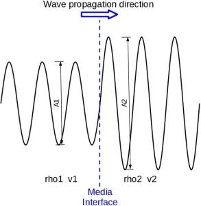
Figure 1: Wave’s transmission through a media interface

Thus, for comparing the seismic energy, using only the amplitude is probably OK if the geophones are all placed at the same layer (the same elastic parameters), which is often the case in surface arrays. However, for downhole arrays, the geophones may be placed at different layers as shown in figure 2. In different layers, the elastic properties are different. In this scenario, if we want to compare the wave energy, it is not suitable for only comparing the recorded seismic amplitude of different geophones. The elastic properties which contribute to wave impedance must be carefully considered.

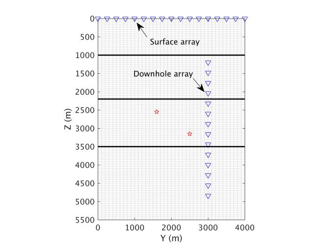
Figure 2: Surface array and Downhole array. With blue triangles show the geophones and red stars show the seismic source.

The references are not very clear and comprehensive. And my knowledge of this are also limited. If anyone could provide any references and corrections, I will be very grateful.

Reference: